
Every catastrophe pricing decision, every economic-capital number for a property portfolio and every reinsurance layer valuation reduces to the same question: what is the distribution of aggregate losses from a class of events over a defined period? The answer decomposes cleanly into frequency, severity and their dependence. The mathematics is well understood; the calibration choices are where models succeed or fail.
This article treats climate and catastrophe risk from the frequency-severity angle. For the actuarial primer see Frequency–Severity Modelling of Insured Catastrophe Losses; for the financial framework linking hazard to loss see Physical Climate Risk; this article focuses on the tail.
The compound Poisson foundation
Let N be the number of events in a period, and X_i the severity of event i. Aggregate loss is S = Σ X_i. If N is Poisson(λ) and the X_i are i.i.d. with distribution F_X, then S follows a compound Poisson distribution. Key moments:
- E[S] = λ · E[X]
- Var[S] = λ · E[X²] (not λ · Var[X])
- Skewness of S depends on the third moment of X
Two features drive most of the modelling debate.
Overdispersion: from Poisson to negative binomial
Empirical event counts in property catastrophe portfolios often exhibit variance in excess of the mean — overdispersion. Physical mechanisms include climate-mode clustering (ENSO, AMO), atmospheric persistence and reporting effects. A negative binomial for N with mean λ and dispersion parameter α > 0 gives Var[N] = λ(1 + αλ), reducing to Poisson as α → 0. In practice α on convective-storm counts and wildfire counts is meaningfully above zero; on hurricane counts it varies by basin and decade.
Heavy tails: the generalised Pareto
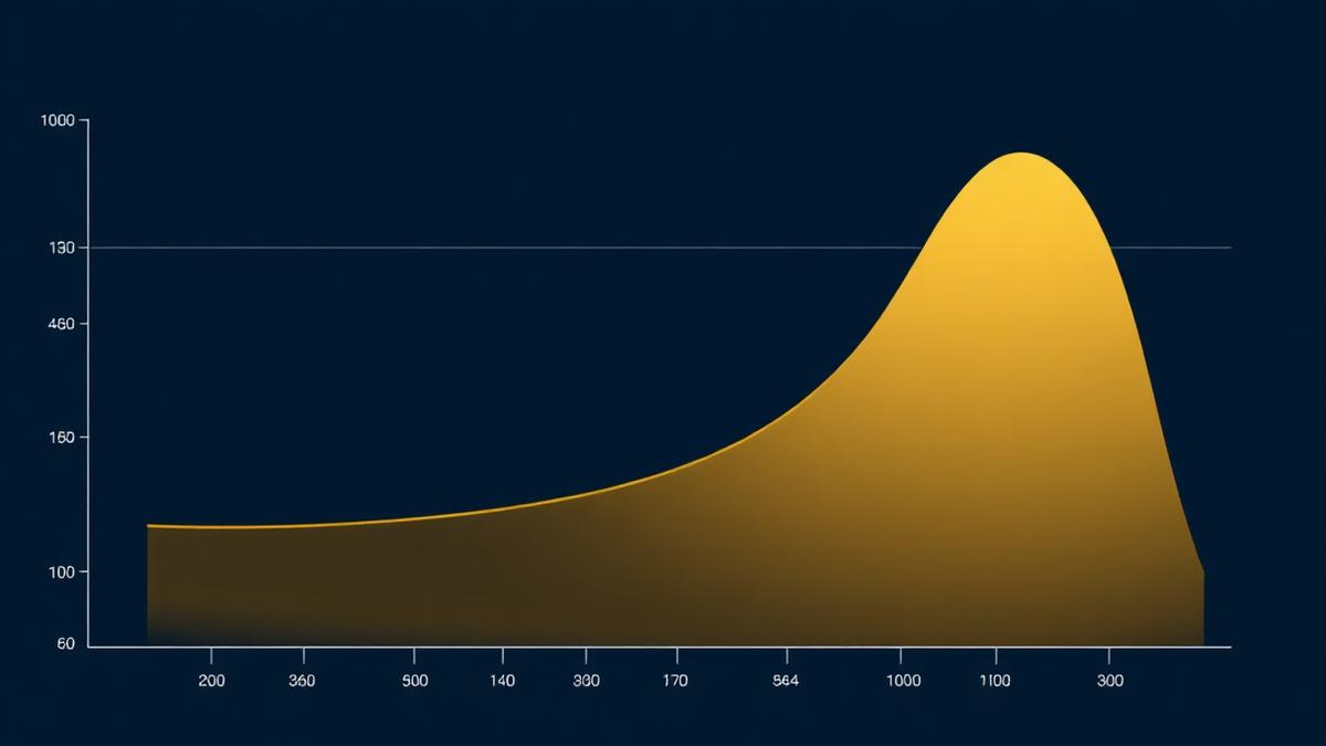
Severity distributions with polynomial tails dominate catastrophe modelling. A common structure is a body distribution (lognormal, gamma) up to a high threshold u, and a generalised Pareto (GPD) above:
F_X(x) = 1 − (1 − F_body(u)) · (1 + ξ (x − u)/β)^(−1/ξ) for x > u
with ξ > 0 the tail-shape parameter and β > 0 the scale. For ξ ≥ 0.5, the second moment of the tail is infinite; for ξ ≥ 1, the mean is. Real catastrophe severity data on secondary perils regularly produces ξ estimates around 0.2–0.4, with wide confidence intervals — the peaks-over-threshold estimation is inherently data-hungry.
Threshold choice is the estimator's Achilles heel. Too low, and the GPD is fitted to the body; too high, and there is not enough data. Diagnostic tools — mean-excess plots, Hill plots — are standard, but a validator should always see a robustness table across three or four candidate thresholds.
Dependence: within event, across peril, across time
Two independent events on the same day are not independent losses if they share exposure. Two events in the same season are not independent counts if a climate mode conditions both. The dependence structure of the aggregate loss is where naive independence assumptions produce the biggest underestimation.
Event footprint dependence. Within a single hazard event, losses across insureds are strongly correlated through the physical footprint. Vendor cat models handle this by simulating physical events on gridded exposure and aggregating losses per event; homegrown models often approximate the same effect with a per-event correlation multiplier.
Cross-peril dependence. Wildfire and drought share climate drivers; convective storm and hail co-occur; flood follows hurricane. Modelling these dependencies via copulas on annual aggregate losses is a defensible compromise between per-event simulation and independence.
Climate non-stationarity. The distribution of event frequency is not constant over decades. NGFS scenarios (see NGFS Climate Scenario Guide) provide long-horizon frequency shifts; near-term calibration should reflect the last 20–30 years, not the last century.
Exposure and vulnerability
The physical hazard by itself is not a loss. Losses arise where hazards meet exposure, filtered by vulnerability. Even a fully specified frequency-severity model on gross physical losses will produce the wrong answer if:
- The exposure database is stale, missing recent construction or aggregating buildings into postcodes rather than coordinates.
- Vulnerability curves — the relationship between hazard intensity and damage ratio — are copied from an unrelated region.
- Policy terms (deductibles, limits, sublimits, event definitions) are applied at the wrong level in the chain.
The chain-form loss formula — hazard → exposure → vulnerability → policy — is set out in more detail in Physical Climate Risk.
Numerical intuition
Consider a hypothetical secondary-peril portfolio calibrated to:
- λ = 10 events per year, negative binomial with α = 0.2.
- Severity per event: lognormal body with median USD 5m, GPD tail above USD 100m with ξ = 0.3, β = 50m.
- No cross-event dependence beyond the frequency clustering.
A Monte Carlo simulation of 100,000 years produces an expected annual loss around USD 200m and a 1-in-250-year aggregate loss around USD 1.8–2.5bn — but the confidence interval on the 1-in-250 number is wide (typically ±30–50%), driven almost entirely by the tail-shape uncertainty. Reporting a single tail number without a confidence band is misleading; the band is the honest signal.
Uncertainty: parameter and model
Two uncertainty sources deserve explicit treatment.
- Parameter uncertainty: the estimation error on λ, α, ξ, β. Bootstrap resampling or a Bayesian posterior distribution provides confidence intervals on the tail metrics.
- Model uncertainty: the risk that the distributional family itself is wrong. Fitting a lognormal-plus-GPD and a mixture of gammas to the same data typically produces different tail metrics at the 1-in-200 level even when both fit the body well.
Ensembling — running multiple models and reporting the range — is standard in weather forecasting and increasingly standard in catastrophe modelling. Vendor-model blending is the industry's version of this principle.
Validation
Validators of catastrophe frequency-severity models should look for:
- Body vs tail fits: goodness-of-fit tests separately on the body and the tail, not just on the whole distribution.
- Threshold sensitivity: how does the 1-in-100, 1-in-200, 1-in-500 change as the tail threshold moves?
- Out-of-sample event replay: does the model, calibrated to pre-2020 data, produce reasonable loss distributions for 2021–2025 events?
- Cross-peril consistency: are correlations between perils calibrated on the same time window as the marginals?
See The Model Validation Lifecycle for the general framework.
Governance implications
Boards should see:
- The expected annual loss, the 1-in-100 and 1-in-250 aggregate loss, and the credible interval on each.
- The sensitivity of the tail metrics to α (frequency overdispersion) and ξ (tail shape).
- The exposure concentrations that drive the tail — usually a small number of accumulations account for the majority of the tail risk.
Where the internal model plugs into economic capital (see Solvency II, ORSA and Economic Capital), the reconciliation to SCR should be documented and reviewed annually.
Limitations
Catastrophe frequency-severity models are as good as the data behind them, and secondary-peril data (wildfire, convective storm, flood) has less depth than hurricane and earthquake data. Non-stationarity — climate change, urbanisation, exposure growth — means the recent past is a biased sample of the near future. Ensembling and honest confidence bands mitigate but do not remove this.
Conclusion
Frequency, severity and tail behaviour together define the shape of catastrophe loss distributions. The models that stand up to scrutiny separate body and tail, quantify parameter and model uncertainty, and align exposure, vulnerability and dependence with the same rigour as the marginal distributions. Everything else is decoration.
Related reading
- Frequency–Severity Modelling
- Physical Climate Risk
- NGFS Climate Scenario Guide
- The Future of Catastrophe-Risk Modelling
References and further reading
- Klugman, S., Panjer, H., and Willmot, G., Loss Models: From Data to Decisions.
- Coles, S., An Introduction to Statistical Modeling of Extreme Values.
- Intergovernmental Panel on Climate Change, Sixth Assessment Report (AR6), Working Group I.
- Network for Greening the Financial System, NGFS Scenarios for central banks and supervisors.
About the author
Part of an ongoing series on catastrophe and climate risk modelling — more about the author.