
Every January, reinsurance pricing teams around the world face the same deceptively simple question: what should a layer of catastrophe cover cost? Not on average over thirty years — this year, for this cedant, for this treaty structure. And despite three decades of vendor catastrophe models and a recent wave of machine-learning enthusiasm, the analytical engine underneath most of those pricing decisions remains the same one actuaries have used for generations: a frequency distribution, a severity distribution, and the discipline to calibrate both honestly.
The relevance of that machinery has, if anything, grown. Swiss Re Institute's sigma 1/2026 puts 2025 insured losses from severe convective storms at USD 51 billion — the third-costliest SCS year on record after 2023 and 2024 — and reports wildfire as the fastest-growing peril, with insured losses rising at an estimated 12% per year (Swiss Re Institute, 2026). These are exactly the perils where frequency–severity modelling earns its keep: many events per year, meaningful data on both counts and sizes, and loss processes evolving quickly enough that a transparent, recalibratable model beats a static one.
The business problem: you need a distribution, not a number
An expected loss is not a price, and it is certainly not a capital requirement. A reinsurer writing a EUR 50 million excess EUR 50 million layer cares about the probability that annual aggregate losses pierce the attachment point, the expected loss within the layer, the volatility loading its capital model demands, and the chance of a full-limit loss. An insurer setting catastrophe budgets cares about the spread of outcomes around the plan. All of these are questions about the shape of the aggregate loss distribution, and the frequency–severity decomposition is the most natural — and most auditable — way to build that shape from data.
The decomposition also matches how the world generates losses. Event counts and event sizes are driven by different physical and economic processes: counts by meteorology and exposure footprints; sizes by intensity, local exposure density, construction quality and claims inflation. Modelling them separately lets each component be calibrated, trended and stressed on its own evidence — a structural advantage no single-distribution fit to aggregate losses can offer.
The model in four symbols
The aggregate annual loss is written as a random sum:
S = X₁ + X₂ + … + X_N
where N is the random number of loss events in the year (frequency) and each Xᵢ is the size of the i-th event (severity), with events assumed independent of each other and of the count. In the classical compound Poisson model, N follows a Poisson distribution with mean λ — the expected number of events per year — and the severities follow a chosen distribution such as the lognormal or gamma.
Two results carry most of the practical weight. The expected aggregate loss is:
E[S] = λ · E[X]
— average event count times average event size. And for Poisson frequency, the variance of the aggregate loss is:
Var(S) = λ · E[X²]
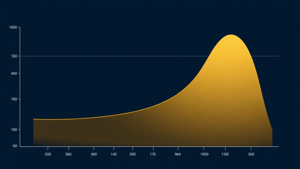
where E[X²] is the mean of the squared severities. That squared term is the whole story of catastrophe economics in one expression: aggregate volatility is driven not by typical events but by the possibility of large ones. Two portfolios with identical expected losses can carry radically different risk if one's severity distribution has a heavier tail — which is why severity-tail assumptions, not frequency assumptions, dominate layer pricing and capital.
Real data usually rejects the plain Poisson assumption for frequency: event counts show more year-to-year variation than the Poisson allows (its variance equals its mean by construction). The standard remedy is the negative binomial distribution, which adds a dispersion parameter to absorb clustering — years where atmospheric conditions produce runs of storms. Testing for overdispersion should be a routine calibration step, not an afterthought; ignoring it understates the probability of bad years even when individual events are modelled well.
Choosing and disciplining the severity distribution
The lognormal and gamma families remain the default severity choices for good reason: both are positive, right-skewed, two-parameter and easy to fit. The lognormal carries a heavier tail than the gamma and often fits large-loss data better; the gamma is frequently more stable for attritional and mid-sized events. But no two-parameter body distribution should be trusted deep into the tail. For layers attaching at high return periods, the honest approach is a spliced model: a lognormal or gamma body below a threshold, and an extreme-value tail — a generalised Pareto distribution — above it. That is the subject of the next article in this pillar, and the splice point itself is a calibration decision that deserves documentation and sensitivity testing.
Calibration discipline matters more than distributional elegance. Before any fitting: losses must be trended to current cost levels (reconstruction-cost inflation has been a material driver of recent loss growth — Swiss Re notes US rebuilding costs remain well above pre-pandemic levels), adjusted for exposure change so that a 2010 event is expressed as if it hit today's portfolio, developed to ultimate where recent events are still settling, and screened for reporting thresholds that truncate the small-loss record. Skipping these steps and fitting to raw losses is the single most common failure mode I see in reviewed pricing work — the resulting parameters are biased in ways no distribution choice can repair.
Worked example: pricing a hail layer
Consider pricing EUR 50m xs EUR 50m aggregate cover for a regional insurer's hail exposure:
- Assemble and adjust: fifteen years of event-level hail losses, trended for claims inflation and portfolio growth, developed to ultimate.
- Fit frequency: annual counts average 6.0 with variance 10.5 — clear overdispersion, so fit a negative binomial rather than Poisson.
- Fit severity: lognormal body fitted by maximum likelihood; QQ-plots checked in the tail; GPD splice tested above the 90th percentile and retained because it materially changes losses above EUR 30m.
- Simulate: 100,000 Monte Carlo years — draw a count, draw that many severities, apply the layer terms to each year's aggregate. (For simple structures, Panjer's recursion or FFT methods compute the aggregate distribution without simulation; Monte Carlo wins once reinstatements and complex terms enter.)
- Read off the economics: probability of attachment, expected layer loss, layer-loss volatility for the risk loading, and sensitivity of all three to the splice threshold and the dispersion parameter.
Every number in that price can be traced to a named assumption. That traceability — not sophistication — is what makes the method durable.
Implications for risk leaders
First, insist that pricing and capital teams present frequency and severity diagnostics separately: an aggregate fit that "looks fine" can hide an overdispersed frequency and an understated tail cancelling each other in the body of the distribution while compounding in the tail. Second, direct review effort at the data-adjustment layer — trending, exposure normalisation, development — because that is where bias enters silently. Third, treat machine-learning proposals for loss modelling as complements, not replacements: ML can sharpen severity predictions from richer covariates, but the compound-distribution architecture, with its explicit assumptions and analytic moments, remains the framework a validator can actually test. At Quantica Risk, our modelling frameworks keep the compound structure as the auditable backbone and confine ML components to clearly bounded roles within it.
Conclusion
The frequency–severity model endures because it mirrors reality's own decomposition — how often, and how bad — and because every one of its parameters can be estimated, challenged and stressed in the open. In a loss environment where secondary perils now dominate annual results and are trending fast, the ability to recalibrate transparently each year is worth more than any black-box gain in fit. The next article takes the one place this framework genuinely struggles — the extreme tail — and shows how extreme-value theory completes it.
About the author. Jonas Osman is a risk-modelling and financial-risk professional and the founder of Quantica Risk, an AI-driven modelling company focused on insurance, banking, climate risk, actuarial analytics, and model validation.
Quantica Risk develops transparent, data-driven modelling frameworks for financial institutions and risk-sensitive businesses. To discuss catastrophe risk, insurance pricing, or model validation, visit the Quantica Risk website. [website — to be inserted when verified]
Series links
- Next in this pillar: Pricing the Tail: Extreme-Value Theory, GPD, and the Market Price of Catastrophe Risk (Article A3) — completing the severity model where two-parameter distributions fail.
- Related: When Perils Compound: Modelling Dependence Across Wildfire, Windstorm, Drought and Heat (Article B3) — what happens when the independence assumptions of this article are relaxed.

References
- Swiss Re Institute (2026). sigma 1/2026 — Natural catastrophes in 2025: the persistent rise of wildfire and storm risk. https://www.swissre.com/institute/research/sigma-research/sigma-2026-01-natcat-2025-wildfire-storm-risk.html
- Swiss Re Institute (2026). Press release, 19 March 2026: Wildfires, storms, floods contribute to record 92% of global insured losses in 2025. https://www.swissre.com/press-release/Wildfires-storms-floods-contribute-to-record-92-of-global-insured-losses-in-2025-says-Swiss-Re-Institute/7b39b1a5-b878-4a55-a5ff-bf5aa561a675
- Klugman, S. A., Panjer, H. H., & Willmot, G. E. Loss Models: From Data to Decisions (5th ed.). Wiley. (Foundational reference for compound distributions, severity fitting and aggregate-loss computation.)
- Panjer, H. H. (1981). Recursive evaluation of a family of compound distributions. ASTIN Bulletin, 12(1), 22–26. (Origin of the Panjer recursion.)
- McNeil, A. J., Frey, R., & Embrechts, P. Quantitative Risk Management: Concepts, Techniques and Tools (rev. ed.). Princeton University Press. (Aggregate risk, heavy tails and dependence.)